Here we offer an overview of one of the most common data structures employed in architectural design education: NURBS.
Overview of NURBS Geometry
History
Technical Specification
Practical Application
Overview of NURBS Geometry
Here we offer a broad-strokes overview of NURBS geometry. Non-Uniform Rational B-Splines, are mathematical procedures of interpolation that are used to represent curves and surfaces.
History
Pierre Bezier
Non-Uniform Rational B-Splines (NURBS) is an amalgam of a number of related and complementary mathematical and computational structures that were progressively developed over time. We may trace the origins of NURBS as far back as the late 1960's, and to the work of Pierre Bezier.
Bezier is the inventor of the Bezier curve, which is the basis of the B-Spline curve, which were later developed into uniform and non-uniform variants. Bezier curves are the simplest of this progression, and hold significant limitations when compared to the NURBS curves we regularly work with in Rhino. Bezier curves cannot, for example, describe simple circles and conics.
NURBS curves may be understood as a more generalizable case of Bezier curves, meaning that a NURBS modeling system is capable of describing a wider range of curves and surfaces in comparison to this previous structure: from straight lines and flat planes, to precise circles and spheres, to piecewise sculptural surfaces. For the purposes of most architectural applications, we may use the terms Bezier Curve and NURBS Curve interchangeably, but with the understanding that the former is a more primitive yet more accessible structure.
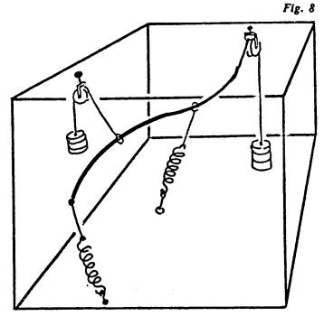
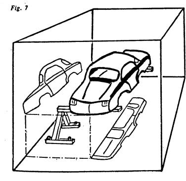
(left) An imagined set of weights and springs. (right) The imagined geometry of a French automobile.
Technical Specification
The Bezier is an interpolation function. This means that given a small set of control points, there is a function that can calculate a smooth transition of points that connect them. Undesirable properties of Bezier curves include their instability for large numbers of control points, and the fact that moving a single control point changes the global shape of the curve. These properties may be avoided by smoothly patching together low-order Bezier curves, which leads us to the generalization of the B-spline. NURBS, in turn, similarly mitigate certain undesirable properties of B-splines.
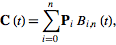
Mathematically speaking, given a set of n+1 control points P_0, P_1, ..., P_n, the corresponding Bezier curve is given by:
NURBS Equation
Using this formulation, Bezier curves that hold any number of control points may be plotted. Quadratic (3-point) and cubic (4-points) Bezier curves are most common. Higher degree curves are more computationally expensive to evaluate. When more complex shapes are needed, low order Bezier curves are patched together, producing a composite Bezier curve (a B-spline or NURBS).
Bezier curves generally follow the shape of their control polygon.
Given n control points, the curve begins at P0 and ends at Pn; this is called the endpoint interpolation property.
The start of the curve is tangent to the first section of the control polygon, and the end of the curve is tangent to the last section.
The degree of the curve is a variable used in the interpolation function, and is typically set to one fewer than the number of control points (setting it higher than this in Rhino will have no effect).
The curve is a straight line if and only if all the control points are collinear.
Some curves that seem simple, such as the circle, cannot be described exactly by a Bezier or piecewise Bezier curve.
A Bezier curve can always be approximated by another bezier curve that has more control points.
There is no local control in degree n Bezier curves - meaning that any change to a control point affects the entire curve.
Equal division along the length of the curve does not correlate with equally spaced parametric division.
Graphic Construction
As we have just seen, the mathematical function for a Bezier curve is a polynomial that takes as input a set of control points, and interpolates values somewhere in between. A remarkably simple algorithm by deCastljau implements this polynomial curve by using only line segments and the basic property that a point on the segment can be evaluated by a parameter between 0 and 1. This is the basis for the elegant algorithm which can be broken down into the following steps, in which we will plot a point on the curve at a given parameter t.
For a clear discussion of this topic from the point of view of a graphic designer, see the excellent Cubic Bezier Curves - Under the Hood video by Peter Nowell.
Connect the control points using line segments in the order specified: P0 should be connected to P1, and P1 to P2, etc.
Evaluate each line segment at the parameter t. Evaluation of a line segment is easy: a t-value of 0.0 will produce a point at the start of the line; a t-value of 0.5 will produce a point halfway along the line; a t-value of 0.75 will produce a point 3/4 along the line. For n control points, this procedure will give n-1 points.
As in step one, connect each of these evaluated points with line segments. This will result in n-2 segments.
Iterate. Continue evaluating points on the last set of line segments and forming a new set of segments until only one segment remains. The point on this last line segment corresponding to the given parameter t is a point on the Bezier curve determined by the control points.
A quadratic Bezier Curve
A cubic Bezier Curve
A fourth-order Bezier Curve
A fifth-order Bezier Curve
A linear Bezier Curve
You can try this yourself in Rhino, as shown in the graphic below (note the discrepancy between a t-value of 0.5 and the midpoint of the curve).
Bezier Construction in Rhino
Parametric Construction
Curves and surfaces are either represented mathematically as explicit, implicit, or parametric. The former two are axis-dependent, cannot easily represent multiple-valued functions, and are very rarely used in CAD and computer graphics. The latter, parametric equations, rely upon a parameter "t" that sets the range of possible values for which the equation may be applied. This range is referred to as the domain.
In summary, there is more than one way to mathematically represent a curve.
Explicit Form
y = f(x)
Implicit Form
f(x,y) = 0
Parametric Form
x = f(t)
y = f(t)
t: a->b
For example, an equation for a circle (of radius 1 and centered on the origin) may be represented in any of these forms. Notice that the parametric definition defines a domain of 0->2pi:
Explicit Form
y = + sqrt(1 - x^2)
Implicit Form
x^2 + y^2 - 1 = 0
Parametric Form
x = 1 * cos(t)
y = 1 * sin(t)
0 < t < 2pi
A Parametric Circle
We may extend this idea to three dimensions. Although the underlying equations are significantly more complex than the ones defined above, NURBS and their antecedents are all parametrically represented. As such, they require a specific domain, and exhibit an underlying u-v grid, just as we see in the sphere example nearby.
(left) A Parametric Surface (right) A Parametric Sphere
Practical Application
There are many CAD software applications that employ NURBS representations in two-dimensions and in three-dimensions: from Rhino to Illustrator, AutoCAD to Revit. While the implementation details of each can vary significantly, and can impact our experience as users of CAD, there are many invariant properties of NURBS that persist. Here we offer an overview of the practical implementation and use of this common data structure.
Control Structures
NURBS Curves and Surfaces are necessarily defined by a lower-level structure: their control points.
There are many conventions for interfacing with these control points, some complimentary (for example, control point "weighting" and "kinking") and some conflicting (for example, the "handle-style" control mechanism in Illustrator vs the "point and end vector" style in Rhino.
Handle-Style
Handle-Style Curve Construction
Handle-style curves allow the author to define locations of important features along the curve, and to control the tangency direction and amount at each. Note that these points are not the control points used to mathematically compute the curve (we can tell because they lie on the curve). Rather, the actual control points are calculated behind-the-scenes in order to produce a curve that passes through the points of tangency as described by the handles. The interface provided by Adobe Illustrator defaults to a handle-style interaction with curves.
Control Cage Style
Control-Cage Style Curve Construction
The 'control cage' style of defining a curve is perhaps less intuitive than the handle-style, since the defined points are not on the curve, but it does hew more closely to actual mathematical calculation of the curve. Here, the user is asked to define a set of control points through which a curve will be interpolated. Note the relationship between the control cage and the resulting curve: only the first and last points given are on the curve, and the points directly adjacent to these describe the direction and magnitude of the tangency (much like a handle).
Kinks and Weights
Special implementations of NURBS can include additional control structures besides the control points - including "weights", or relative influence of each point, and "kinks" indicating a moment of non-tangency.
Features and Idiosyncrasies
Due to their nature as interpolated parametric descriptions, NURBS Curves and Surfaces present a number of features that we might expect as well as idiosyncrasies that we might not.
Directionality
NURBS curves have a direction
Because they are described by parametric equations, NURBS curves and surfaces exhibit directionality. When working with curves to create higher-level objects we must be aware of their relative directions. Use the Dir command in Rhino to view and edit the direction of objects.
Non-Uniform Division
NURBS curves are not naturally divided into equal-spaced segments
Also due to their parametric nature, the division of NURBS curves and surfaces into equal-length divisions is not a natural operation. While software packages such as Rhino offer methods for doing so, such as the Divide command, other processes (such as the Grasshopper division of a curve seen nearby) suffer from the non-uniformity of NURBS curves.
Rectangular Topology
NURBS Surfaces are four-sided. Always. Their u- and v- directions are revealed to us when we view the isoparametric lines (or isoparms) that inscribe the rectangular grid on them. Dealing with the four-sided nature of the NURBS surface is like working with a rubber sheet. There are a number of approaches to sidestepping the four-sidedness of NURBS Surfaces, but each of these should be taken with a grain of salt. These are, in essence, "wrappers" or hacks, and the underlying mathematical representation of the NURBS Surface remains four-sided in each of them.
Subdivide
A non-four-sided figure may be subdivided into four-sided parts.
The most direct approach to getting around the four-sided limitation is to subdivide a given surface into four-sided parts. This generally works quite well, as the integrity of the NURBS surface is maintained. However, it can be ineffective in describing certain classes of form, and difficult to maintain if edges are forced into locations where they are not required.
Shrink
We may describe a three-sided figure using a four-sided structure by "srinking" one of the sides to a point.
Shrinking an edge of a NURBS surface until it's dimension is nearly zero is another approach to the four-sided limitation, one that allows the construction of something that is topologically triangular. The downside of such an approach is that isoparametric lines will converge toward the "shrunken" edge. This can cause problems when arraying objects along the surface, or using the surface as a guide for the positioning of dependent geometry.
Stretch
It's not pretty, but one edge of a NURBS surface may be stretched and distorted such that it approximates two edges of a figure. The corner that lies at the middle of one of the NURBS surface edges will always display a rounded corner of some dimension.
Trim
By employing the higher-level description of a curve that rides along the surface of a NURBS Curve and defines a "legal boundary" beyond which the surface is simply ignored, we can create NURBS Surfaces with however many sides we want. The unfortunate consequence of this approach is that edits to the underlying surface must be conducted separately from the trim curve, which often results in difficult situations along trimmed edges.