Here we offer a discussion of the two key types of data that structure graphic information in the computer. These two types, raster data and vector data, are used on their own, or can also be combined, in the service of expanding the reach of the pure black lines on white paper that characterize classical graphic projection drawings.
Vector Graphics
The Structure of Vector Graphic Data
Salient Features and Issues
Raster Images
The Structure of Raster Data
Salient Features and Issues
Hybrid Structures
There are two fundamental ways to describe two-dimensional graphics using computers:
Raster images (sometimes simply called "images" or "pixel-based graphics")
Vector graphics (also referred to as "artwork" or "object-oriented graphics").
Understanding the nature of these two data structures, and the benefits and drawbacks of employing each, is fundamental to the effective use of computing in visual design.
Vector Graphics
Vector graphics is an approach to representing graphic information using lines, polygons, and interpolated forms defined in Cartesian coordinates (the x and y axes implied by the rectangular frame of most digital media).
Under this approach, all drawn shapes are expressed as discrete entities defined by locations on the screen, along with other numeric properties such as radii, fill and stroke color, and line weights.
Due to this data structure, and because forms are described procedurally rather than explicitly (E.g. "draw a circle of this size here, and then draw a rectangle of this dimension there"), vector graphics have the ability to render type and large areas of color with relatively small file sizes. They can also be reduced or enlarged to any size without losing any image quality.
The Structure of Vector Graphic Data
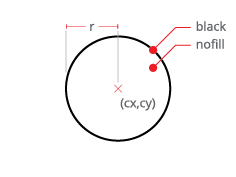
A vector graphic is stored as a list of independent shapes and their salient properties. Each shape is described in terms of the procedure required to draw it. For example, consider the vector representation of a circle.
The pieces of information required to draw this circle might include:
an indication of the type of shape (circle)
the radius r
the location of the center point of the circle
stroke line style and color (possibly transparent)
fill style and color (possibly transparent)
In a hypothetical vector data file, we might expect to find a description of a circle that includes the pieces of information described above. Indeed, if we examine the specification of a circle in an SVG file (SVG stands for "scalable vector graphics", and is a popular format for displaying vector information on the web) we find just this:
When such a file is rendered by our web browsers, it is displayed like this:
Vector graphics can include many different types of objects, including lines, boxes, circles, curves, polygons, and text blocks. All these items can have a variety of attributes--line weight, type formatting, fill color, graduated fills, and so on.
When working with vector graphics in architectural design, we should be aware of the following features, advantages, and limitations in comparison to raster formats.
File Size
Describing forms using a minimal amount of information allows for much smaller file sizes in comparison to raster images. instead of describing a rectangle with thousands (or millions) of dots, vector graphics just say, "Draw a rectangle this big and put it here." Clearly, this is a much more efficient and space-saving method for describing some kinds of art, but not others. The file size of a vector graphic is directly proportional to the number of shapes represented. We can see this in the way that PDF files containing a few shapes are quite small, while ones that contain a great many shapes get very large.
Scalability and Editability
Because each primitive form is described in terms of the processes necessary to draw it, these forms may be scaled to any size without losing detail or fidelity. Similarly, Since vector shapes are described in terms of the parameters required for their creation, these are stored in the data file and may be easily modified. This allows for the transformation (moving, scaling, rotating, filling) of the logical elements of each graphic.
Draw Order
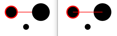
Since a vector graphic is expressed as a list of independent shapes, the order in which each shape appears in this list can have an effect on the resulting image. To illustrate, consider the following SVG code:
This code produces the image on the left, below. Can you imagine what changes would be required to alter the code to produce the image on the right? Try modifying this example using the CodePen Online Editor.
For a complete SVG reference, including a list of shapes available, see the SVG Reference.
Raster Images
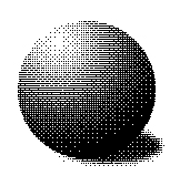
Raster images (sometimes called pixel-based graphics or bit-mapped graphics) are constructed from grids of tiny squares, each a single solid bit of color.
If we look closely, we can see that much of the physical output of digital media is structured in this way, including the pixels on our computer screens and televisions and the tiny dots of color produced by inkjet printers. Beyond these means by which digital media is expressed physically, this technique is also very commonly employed as way of describing graphics digitally, and forms the foundation of raster-based data files, raster manipulations, and image-editing software.
For each of these purposes, data is structured in order to define the graphic qualities of each pixel in a grid.
The Structure of Raster Data
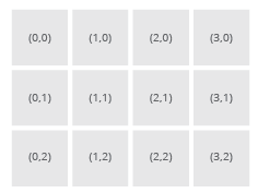
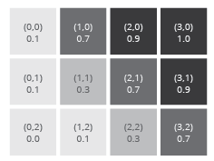
Raster image files consist of a single entry for each pixel of the image described. In this table of entries, each pixel is assigned an address, which we might imagine is like an x-y coordinate that starts with (0,0) and proceeds through all the rows and columns of pixels in the image. By convention, these are numbered starting at the top left, and proceeds from left-to-right and from top-to-bottom.
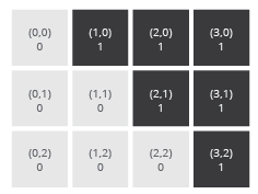
(left) A raster grid of pixel addresses. (right) Simple pieces of information stored in an addressed grid.
In the file and in computer memory, each of these numbered pixels is related to some piece of information.
In the simplest case, we can image that each pixel may hold one of two values: a "0" if it should be drawn as white and a "1" if it should be drawn as black. Such an image would be referred to as a binary image or a two-color bitmap. Images such as this are rarely used in architectural design, but are common stepping-stones in larger processes in digital image processing.
For some simple examples of binary images, see any of the sample PBM files provided. For some simple examples of linear gradient images, see the sample PGM files provided.
What's in a Pixel?
Given a raster data structure, nearly any type of graphic information can be stored in each pixel, ranging from the exceedingly simple 1 or 0 found in a two-color bitmap, to a host of approaches that are employed in describing color (that we discuss below). There are a surprising range of variations on this basic structure. For example, not every image is configured to describe square pixels, and applications exist that support rectangular and even hexagonal grids of pixels. More striking is the fact that raster data structures are used to describe things other than images, with a grid of pixels used to hold higher-level digital forms that are well-described as a grid of discrete objects, such as the vectors in a discrete vector field.
We focus here on those approaches to describing an image using fields of pixels each of a single color, which, on a basic level, we may understand as being represented by a binary (0 or 1 for each pixel), a linear gradient (any value between 0 and 1 for each pixel), or by some representation of color. This brings us to the topic of how color is described digitally.
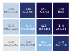
(left) A raster grid of tonal values. (right) A raster grid of RGB values.
Color Spaces
There are a number of models for describing a color in digital media, each of which was developed with a specific application in mind, and was crafted to best serve its intended use.
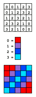
Indexed Color
Indexed color is among the simplest representation of a color in a raster image. It is a technique to manage colors in order to save computer memory and file storage. When an image is encoded in this way, color information is not directly carried by the image pixel data, but is stored in a separate piece of data called a palette: a table of colors. Every element in the array represents a color, indexed by its position within the table. Here, the image pixels do not contain the full specification of a color, but only its index in the palette.
Explicit Color
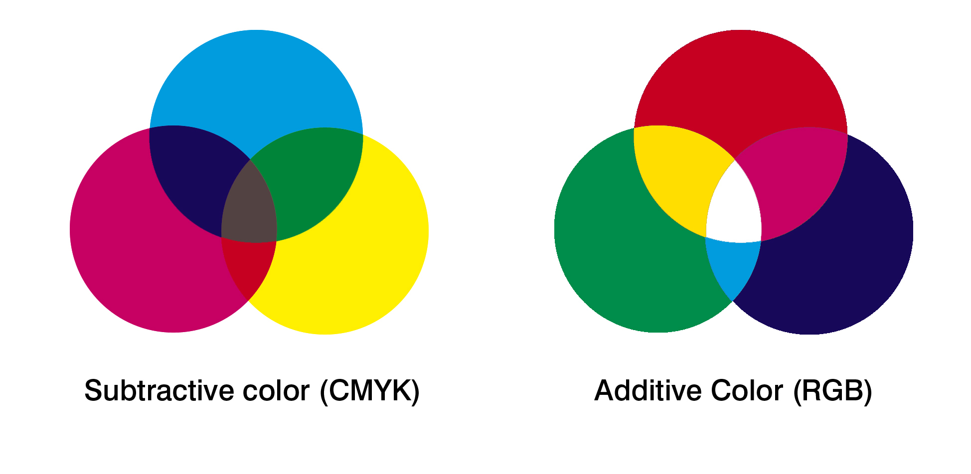
Beyond the indexed approach to representing colors using indices in a table, most other color spaces employed in architectural design represent the color of each pixel explicitly. A primary distinction among the color models discussed here is that of additive colors (most often described by the RGB space) and subtractive colors (most often represented by the CMYK space). The difference between these two has to do with the intended medium in which we are working. When we mix colors using paint, or through the printing process, we are using the subtractive color method. Subtractive color mixing means that one begins with lightness (the paper) and ends with darkness (the pigment); as one adds color, the result gets darker and tends to black. If we are working in a projected or emitting medium, the colors we see on the screen are created with light using the additive color method. Additive color mixing begins with black (an inactive pixel) and ends with white (a fully light pixel); as more color is added, the result is lighter and tends to white.
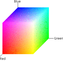
RGB
Stands for Red, Green, Blue, and is the closest to the way that our computer monitors understand color. This is the dominant model for describing additive colors, and is widely used in the sensing of color (such as in digital cameras) and in the representation of colors (as in computer monitors, televisions, and projectors). In additive color models such as RGB, white is the "additive" combination of all primary colored lights, while black is the absence of light.
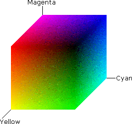
CMY / CMYK
Stands for Cyan, Yellow, Magenta, and sometimes blacK, and is the closest to the way that our printers combine basic ink colors to print images and drawings. This is the dominant model for describing subtractive colors, and is directly applied in the mixing of pigments for printing and painting. The CMYK model works by partially or entirely masking colors on a lighter, usually white, background. The ink reduces the light that would otherwise be reflected. Such a model is called subtractive because inks "subtract" brightness from white. In the CMYK model, colors in generated in the inverse process of additive systems: white is the natural color of the paper or other background, while black results from a full combination of colored inks. To save cost on ink, and to produce deeper black tones, unsaturated and dark colors are produced by using black ink instead of the combination of cyan, magenta and yellow.
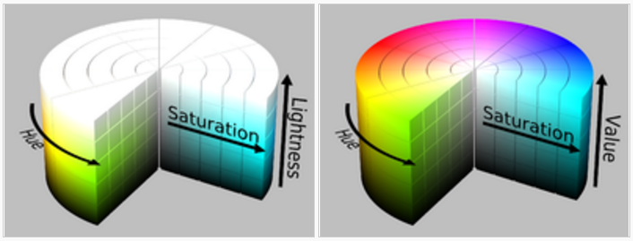
HSB / HSL
Stands for Hue, Saturation and Brightness (sometimes called value, resulting in the HSV acronym) and Hue, Saturation and Lightness (and is sometimes called HLS) respectively. These closely-related color spaces were developed as an alternative to RGB that presents more intuitive and perceptually relevant results.
Lab
Stands for Luminance (lightness), "A" and "B" that are chromatic components (A ranges from red to green, and B ranges from blue to yellow). This color space, while decidedly less prevalent than others listed above, exceeds them in that it includes all perceivable colors, which means that its gamut is more generous than those of the RGB and CMYK color models.
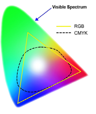
Relative Gamuts of Prevalent Color Spaces
Not all color spaces are alike, and different color spaces are differently able to capture portions of all colors perceptible to humans. The term color gamut is used to describe the extent of the set of colors able to be described by a given color space. In most cases, this set is a smaller subset of all those colors we are able to see.
As shown in the nearby graphic, the typical CMYK color space is able to capture a smaller region than the typical RGB system. While smaller overall, this region does include colors that are not included in the RGB gamut. This means that when converting between the two spaces, we may expect some changes to the colors we are working with.
Layers and Channels
Most software packages allow us to inspect and combine the information contained in the pixels of a raster image in various ways. Among the most prevalent of these are the separation of channels and the superimposition of layers.
As we have seen in the description of color spaces above, a single color is very often comprised of a collection of smaller elemental values. A color described in RGB space is composed of red, green, and blue components while a color described in CMYK space is comprised of similar elements. Most image editing software allows us to inspect and manipulate each of these elements (or channels) at a time for any given image.
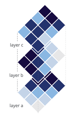
Layers
Many raster image editing software employs a layer structure, which is similar to a "stack" of overlaying raster images on top of one another. When so structured, new issues arise, such as the ordering of layers (which is on top and which is below) and strategies for combining individual layers together to form an image.
Salient Features and Issues
When working with raster images in architectural design, we should be aware of the following features, advantages, and limitations in comparison to vector formats.
File Size
The file size of raster images is in direct proportion to the number of pixels stored, and the amount of information required by each pixel. Given an identical number of pixels and type of data stored, any two raster files saved in an uncompressed format (such as PNG or uncompressed TIFF) will take up exactly the same amount of space on your hard drive, no matter the image depicted. Other formats (such as PNG, GIF, and JPG) store their data in a manner that allows for leaner storage, depending on the specific features of the image.
Resolution and Dimension
Notice that throughout our discussion of raster images, we have not yet mentioned any explicit description of dimension outside of the number of pixels contained in an image. This is because, besides these pixels, there is nothing inherent to a raster image that would relate it to any particular physical size.
Like most digital descriptions of form, raster images are inherently dimensionless in physical terms. This is not to say that physical dimensions cannot be assigned to images, but rather that, unlike a description of their pixel grids, such assignments are not essential to the image itself. The relationship between physical dimension and pixel count is called the resolution or the pixel density of the image.
In most image editing programs we are able to assign and manipulate both physical dimensions and pixel dimensions independently. Most also offer methods for altering these two quantities at the same time. To better understand the issues surrounding image resolution and dimension, let's clearly define some terms:
Pixel Dimension
The number of pixels in the image, usually described as the number of rows by the number of columns of pixels. When we refer to the image as "640 by 480" or "1024 by 768", these numbers typically refer to the pixel dimension. When this quantity is altered, we must recompute the underlying data of the image, either inventing new information (when enlarging an image) or reducing information (when shrinking an image) to fit.
Physical Dimension
An applied quantity that describes the intended width and height of the image when presented or transferred to a physical medium, such as when printing. This quantity may be altered without necessarily affecting the underlying data of the image.
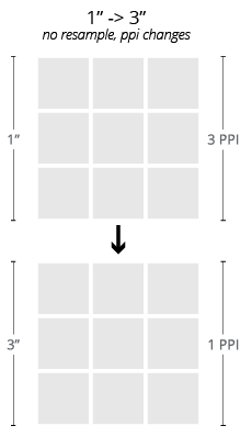
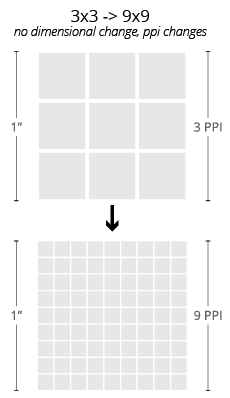
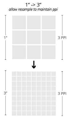
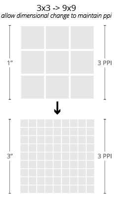
Resolution (pixel density)
The relationship between the pixel dimension and the physical dimension of an image. This is always described as a ratio, and typically expressed in terms of pixels per inch for a single dimension (the number of pixels in a row per linear inch of image). While this is more appropriately termed the PPI of the image, the acronym DPI (dots per inch) is inherited from the printing terminology and is very commonly employed as well. In metric, we might see this quantity expressed as pixels per centimeter (PPCM).
Since it is a ratio, altering the resolution of an image requires that we alter the pixel dimension, the physical dimension, or both. This fact is easily overlooked, but holds important ramifications to the images we work with regularly as designers (as demonstrated nearby).
Raster-Vector Hybrids
Most graphic software we use has been developed with one of the two models presented above - raster or vector - in mind. Adobe Illustrator is a vector graphic editor, while Adobe Photoshop is a raster image editor.
Similarly, graphic file formats have been developed to store one of these two categories of graphic data:
PDFs and SVGs are formats designed to hold vector information
JPGs, PNGs, GIFs and TIFFs are designed to hold raster information.
Since the inception of these softwares and file formats, however, features have been developed that have blurred the line between these two elemental forms.
Adobe Illustrator now offers features that integrate raster images into a canvas dominated by vector artwork, and even offers Photoshop-style filters that may be procedurally applied to vector artwork that begin to imitate raster-like effects (such as blurring).
Adobe Illustrator, despite being a vector graphics editor, also offers raster-based effects. These sorts of hybrid features "blur" the lines between raster and vector.
Similarly, Photoshop now incorporates vector "layers" that can interact with raster information, and which function much like vector objects in Illustrator. The file formats originally designed to store vector or raster information similarly have since been developed to offer limited support for both models.


